Adding Multiple Dispersions with Multiple Inflows
This section will setup and run four dispersion simulations based on the ventilation results reviewed in the last section.
-
From the Add Items tab, select Dispersion Simulation from the dropdown menu.
-
Use the Ctrl+Click method to select BOTH the North-Easterly, 5 m/s and Easterly 5m/s simulations from the Ventilation dropdown menu, as in Figure 20. You may have to un-select the Westerly default option.
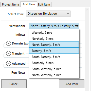
Tutorial 5 - Figure 20 - Selection of the North-Easterly and Easterly wind simulations.
-
Choose the HP Release 02 as the Inflow, you may have to click off the dropdown menu to confirm selection of just one inflow. Note that if we wanted to run HP Release 02 and HP Release 03 with the same ventilations, we would only have to select both inflows for this step. Meaning that the 2 ventilations with the 2 inflows for this step would produce 4 dispersion cases, feel free to do this in your own working project file.
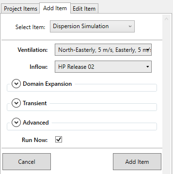
Tutorial 5 - Figure 21 - Setup for 2 dispersion cases of 'HP Release 02 on North-Easterly' and 'HP Release 02 on Easterly'
-
Leave the Mesh Expansion, Transient, and Advanced options as-is for now.
-
Ensure that the Run Now checkbox is selected and click the Add Item button
-
Repeat steps 1 through 5 selecting the Northerly, 5 m/s and North-Easterly, 5 m/s ventilation simulations for the HP Release 03, as shown in Figure 22 and Figure 23 below.
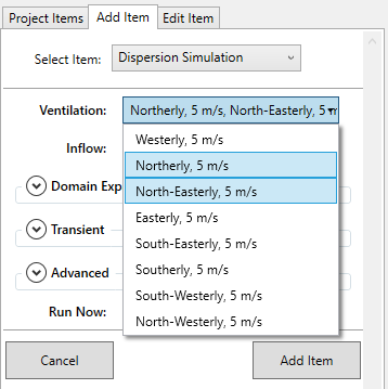
Tutorial 5 - Figure 22 - Selection of the Northerly and North-Easterly wind simulations
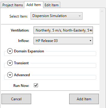
Tutorial 5 - Figure 23 - Indication that both Northerly and Norther-Easterly winds have been chosen with the HP Release 03 for the new dispersion cases
-
Look at the Project Items tab to ensure that four additional dispersion simulations have been added.
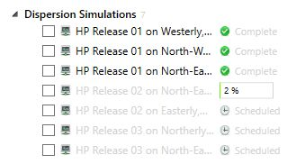
Tutorial 5 - Figure 24 - Showing the four new dispersion simulations added to the project
-
That's it! You have now set-up four new dispersion cases for a total of 7 CFD simulations set-up in this tutorial alone. Let each of the simulations finish calculating before continuing. Have a look at the meshing and contours of variables as the calculation progresses via the Simulation Monitor by double-clicking the case you want to view.
-
Once completed, open the Monitor Point Data window and take a look at the %LFL values for the new simulations. As there are over 28 points in the project, it becomes difficult to discern where the important data is.
-
One helpful trick is to export the selected variable to Excel and adding some Conditional Formatting to color the cells based on their values. Figure 25 below shows an example of Conditional Formatting being used with exported monitor point data for this tutorial to discern which points are most relevant to this example. Notice how 'Monitor Point Grid 08' has all values of 0. This is because when monitor points were added using the area spacing function, this point was placed inside one of the vessels. As seen in Figure 26.
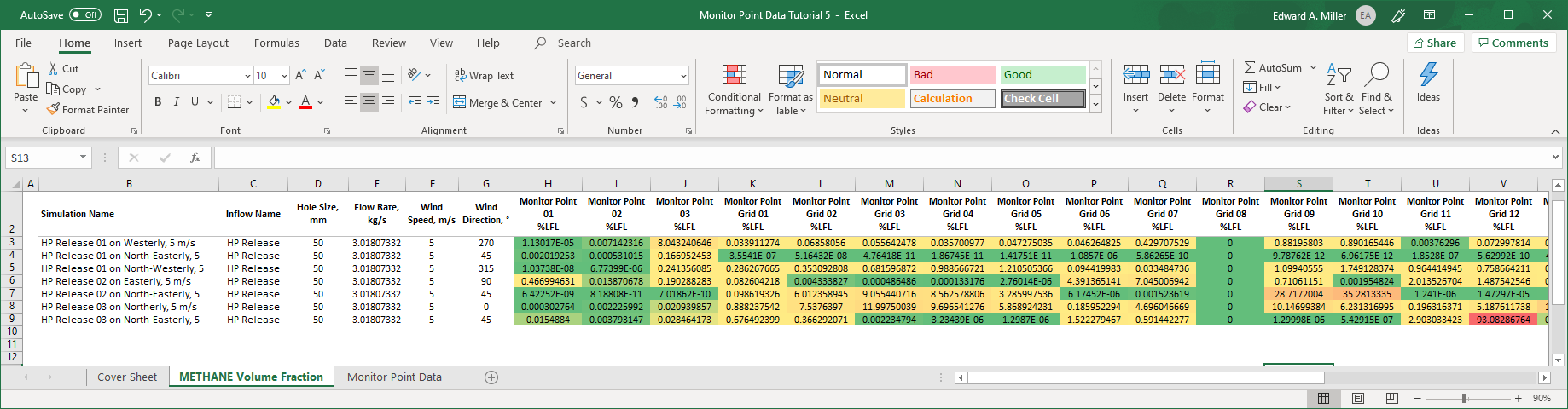
Tutorial 5 - Figure 25 - Excel export with conditional formatting for the Methane %LFL of the completed dispersion simulations.
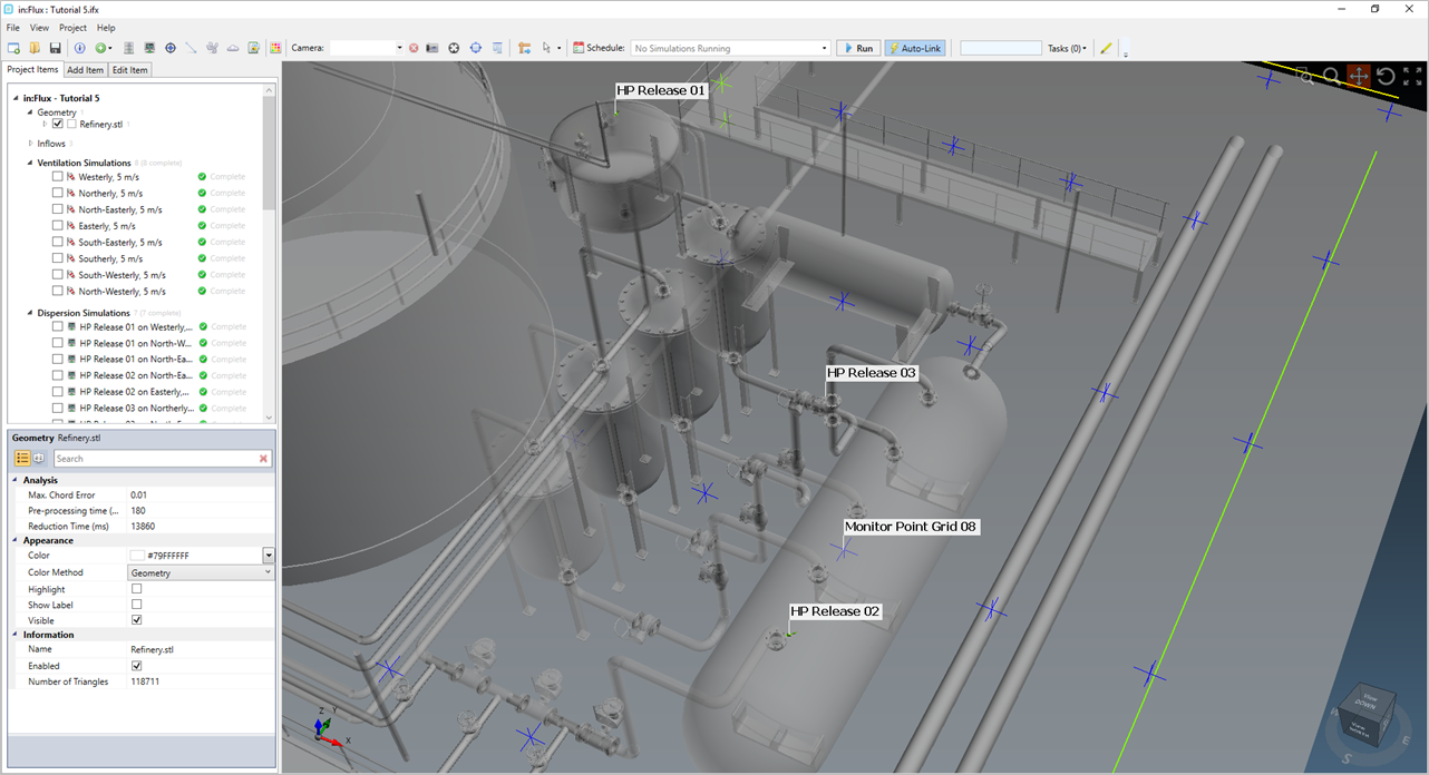
Tutorial 5 - Figure 26 - Determining that Monitor Point Grid 08 location is indeed inside the large horizontal vessel. The transparency of the geometry was changed to generate the figure.
The exported excel document in Figure 25 was used to choose the following monitor points in the Monitor Point Data window shown in Figure 27. Each was selected by searching for cells in the excel with higher %LFL value. Figure 27 was then created by selecting the associated monitor points from the Points dropdown menu. We can see in the table that HP Release 03 on North-Easterly, 5m/s results in Monitor Point Grid 12 having a value above 100%LFL, which means the air here has a higher than 4.4% concentration of methane. This is also the largest value obtained by the monitor points for the 4 simulations of this tutorial. In the next section we will look at the isosurface for this simulation to confirm these values.
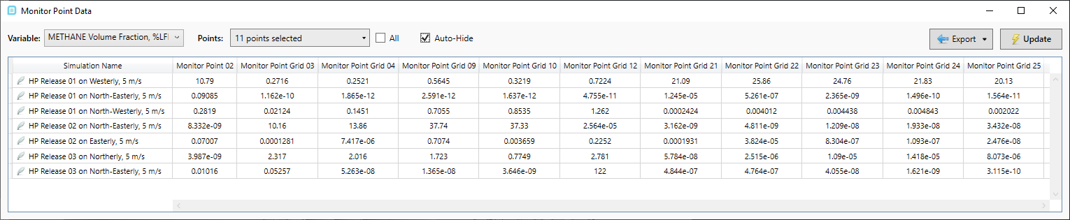
Tutorial 5 - Figure 27 - %LFL concentration values for the new dispersion cases
-
-
Now take a look at the gas cloud analysis data for the entire facility, shown in Figure 28 below, we see that HP Release 02 on North-Easterly, 5 m/s, HP Release 02 on Easterly, 5 m/s and HP Release 03 on North-Easterly, 5 m/s generates the highest values for volume of gas. It is important to look at all the gas cloud data as well as the monitor point data as the monitor points give a spot measurement at a specific height while the monitor region looks at the total volume of gas. Look at the other Monitor Regions (shown in Figure 29 and Figure 30 below) to see that for the more localized regions that HP Release 03 on North-Easterly, 5m/s case produces the largest gas cloud for all the cases run.
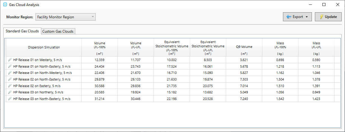
Tutorial 5 - Figure 28 - Gas Cloud Analysis window showing volume size for newly completed simulations compared with previously calculated simulations

Tutorial 5 - Figure 29 - Gas Cloud Analysis window for Lower Flanges Monitor Region
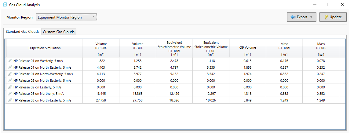
Tutorial 5 - Figure 30 - Gas Cloud Analysis window for Equipment Monitor Region
Continue to the next section to look at isosurfaces of the newly added dispersion simulations.