‎ Adding New Monitors and Reviewing Data

 

in:Flux was designed to allow users to continue work on the project while simulations are running. Inflows, visualizations, monitor points, monitor lines, monitor regions, new ventilation and dispersion cases can all be added while calculations are completing.

 

In this section, we will add a new monitor line along the northern perimeter of the facility. Like in Tutorial 3 we can use the monitor line to assess gas detector positioning, in this case an open-path detector.

 

1. Click the Add Item tab and select Monitor Line from the dropdown menu

2. Change the Name to "Monitor Line - North Perimeter"

3. The pick tool will be used to obtain the x and y coordinates for the two opposing points of the line (Start Point and End Point) and then a z-coordinate will be manually entered to raise the monitor points above the ground.

   1. Right-Click in the 3D window and from the View From option select Top View.

   2. Use the pick tool for the Start Point and select a point on the ground north of the western tank, or manually enter "(-32, 43, 2)"

   3. Use the pick tool for the End Point and select a point slightly southeast of the southernmost flange or manually enter "(20, 43, 2)" as shown in Figure 04 below.

       

      

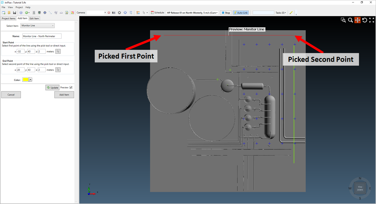
      Tutorial 5 - Figure 04 - Points to select for first and second locations of the new line spaced monitor points.

       

   4. If you used the pick tool, change the z-coordinates of both points to be "2" so that the line is two meters above the ground.

4. To match the other monitor line, set the Color to Yellow by clicking the color dropdown menu and selecting the yellow swatch () from the color palate.

5. Check the Preview checkbox to ensure the points are in similar locations as Figure 04 and Figure 05.

6. Click the Add Item to add new monitor line to the project.

 

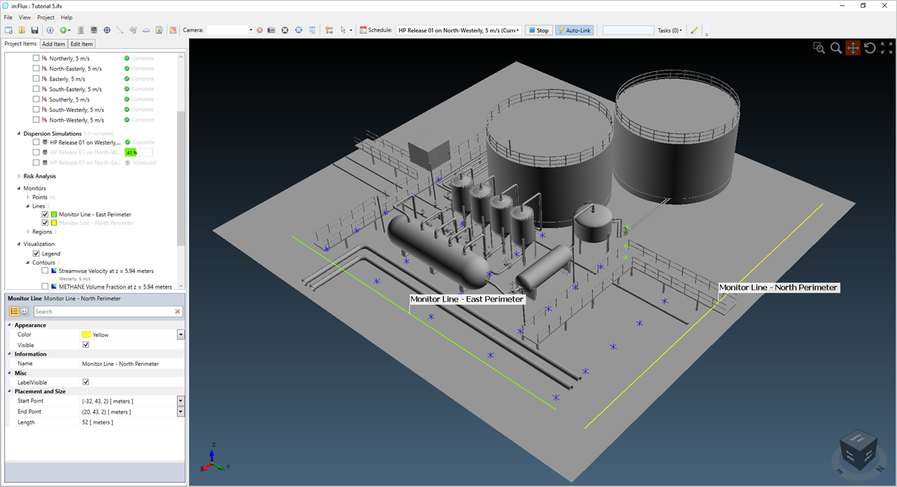
Tutorial 5 - Figure 05 - Placement of the ten additional monitor points near the lower flanges of the facility.

 

Note that in Figure 05 above, in the Project Items tab, the new name "Monitor Line - North Perimeter" will have a gray text as they have not been updated with the most recent simulation data.

 

Open the Monitor Line Data window by clicking Monitor Line Data from the Project menu or select the icon on the toolbar. The newly added monitor lines will already be listed in the window. Remember, you are not limited to the number of monitor points, monitor lines or monitor regions that you can add to a project. The only limitation is the time it takes for in:Flux to extract the data from memory.

 

Press the Update () button in the Monitor Line Data window. 

 

Depending on the completion of your simulations, Figure 06 shows the HP Release 01 on North-Westerly added to the Monitor Line Data window which shows the Average Streamwise Velocity across both of the monitor lines. Switching to the Min Value as the Type will show us that there are negative values for the flow along the monitor line, meaning that the flow is in the opposite direction of the defined wind. This can be verified by looking at the vector field or contour of the streamwise velocity for each wind case.

 

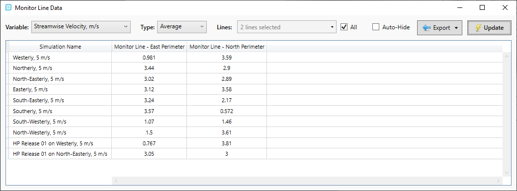
Tutorial 5 - Figure 06 - Updated Monitor Line Data for each of the ventilation cases

 

Newly completed dispersion simulations will automatically appear as a new row in any of the monitor windows and have values for ALL the variables listed in the Variable: dropdown menu. If a monitor is added before a simulation completes then it will automatically contain the needed data. If the monitor is added after a simulation has completed, it will need to be updated.

 

When looking at variables related to gas dispersion such as %vol, ppm, LFL, %LFL, %UFL, etc the ventilation simulation rows will not have any relevant data and will appear with a "-", as shown in Figure 07. This is applicable to both Monitor Points and Monitor Lines. For these cases, click the Auto-Hide checkbox at the top of the window and the rows without data will be visibly removed, as seen in Figure 08. Note that METHANE Volume Fraction, LFL is used and not %LFL as the integrated value gives us the variable per meter, thus Figure 07 and Figure 08 values are in LFL.m.

 

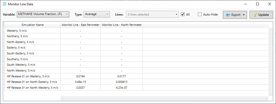
Tutorial 5 - Figure 07 - Showing 'METHANE Volume Fraction, LFL' which for the 'Integrated' values represents LFL.m, also apparent is the lack of data for the ventilation simulations.

 

 

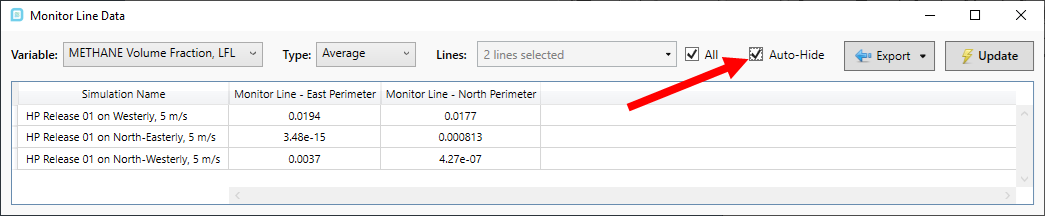
Tutorial 5 - Figure 08 - View of Monitor Line Data window when Auto-Hide is selected for the LFL variable.

 

Open the Gas Cloud Analysis window by clicking the cloud icon () on the toolbar or selecting Gas Cloud Analysis from the Project menu. Figure 09 below shows that, for the three simulations that have been completed, the 'HP Release 01 on North-Easterly, 5 m/s' case has the largest gas cloud. Both of these tables (Figure 08 and Figure 09) will be something to keep watching as more dispersion cases are added.

 

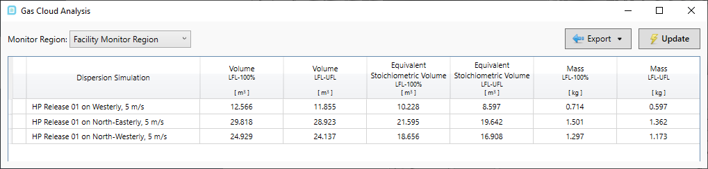
Tutorial 5 - Figure 09 - Gas cloud data window showing information for the three completed simulations for the Facility Monitor Region

 

 

Even if your machine is still calculating cases, you may continue on to the next section to add an inflow. Optimizing your time is easy with in:Flux, there is no need to wait for all simulations to complete before working on other parts of the project.