Reviewing Transient results with ESD, BD and Inventory
Visualizations for simulations with shutdowns, blowdowns and inventory can be setup and viewed in the same way as with transient simulations described earlier.
Let the simulations finish calculating if they have not already.
Open the Monitor Point Data window and see the completed simulations and set the Variable to Methane Volume Fraction, %LFL. Notice how the Monitor Point 03 cell is much lower than in the previous section for the HP Release 01 with ESD case.
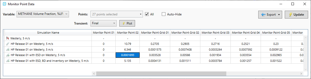
Tutorial 8 - Figure 26 -Monitor Point Data window containing the dispersion case with a shutdown
Double-click the Monitor Point 02 cell indicated above to show the graph of %LFL vs time. The concentration increases with time until right after the shutdown then quickly dissipates from the wind. After 10 seconds the concentration drops off as the gas cloud is dispersed away from the monitor point by the westerly wind.
![]()
Tutorial 8 - Figure 27 - Graph of Monitor Point 02 data for a dispersion with a shutdown
The graph with the 'Link' icon (![]() ) selected will ALWAYS show the data for the cell selected in
the Monitor Point Window. De-selecting the Link box will allow you to double-click on another cell and view a second graph. Figure 28 below shows how you could compare the steady state data with the transient %LFL data at Monitor Point 02.
) selected will ALWAYS show the data for the cell selected in
the Monitor Point Window. De-selecting the Link box will allow you to double-click on another cell and view a second graph. Figure 28 below shows how you could compare the steady state data with the transient %LFL data at Monitor Point 02.
-
Double-click on the cell corresponding to Monitor Point 02 and the HP Release 01 data
-
The graph will appear showing the increase of %LFL to above 11%LFL at 40 seconds
-
Click the 'Link' button to un-link the graph to the selected cell in the monitor point data window (making it not blue)
-
Double-click on the cell corresponding to Monitor Point 02 and HP Release 01 with ESD.
-
A second graph will appear corresponding to cell selected in part d.
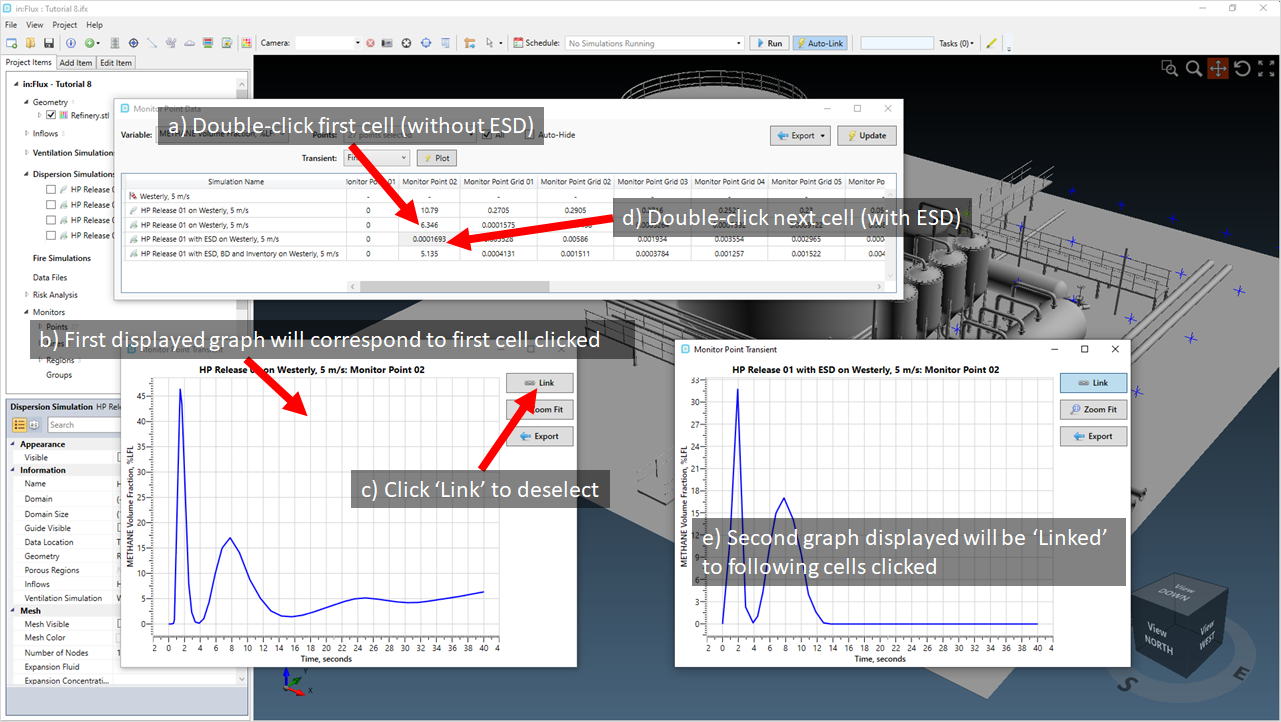
Tutorial 8 - Figure 28 - Process of un-linking graphs to compare simulation data
Using the steps mentioned above, you can quickly compare results from different cases or different monitor points, e.g. the ESD case to the results of the ESD with inventory.
Any of graph seen using these methods can be exported to Excel with its tabulated data. You may also right-click within the graph and save it as an image or copy it to your computer's clipboard.
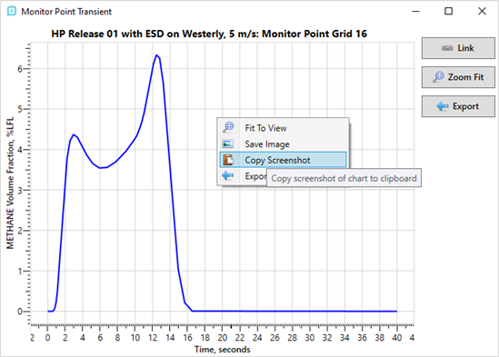
Tutorial 8 - Figure 24 - right-click menu within the transient graph window to save the graph as an image or copy to the clipboard
You have now completed Tutorial 8 and have an understanding of transient simulations in in:Flux. Save you project file once you are done reviewing.