Setting up and Running a Dispersion
A dispersion simulation in in:Flux is defined by combining one ventilation simulation with one inflow. Once the process of defining inflows and ventilations is understood, hundreds of dispersion simulations can be set up to run in just a matter of minutes, this will be discussed in more detail in Tutorial 5.
To setup a dispersion simulation, select a wind simulation to use with the already defined inflow:
-
Click the Add Item tab and select Dispersion Simulation from the dropdown menu.
-
All ventilation simulations for the project will be listed in the Ventilation dropdown menu. As only one has been set up, Westerly, 5 m/s should already be selected for you.
-
Similarly, inflows of the project will be listed in the Inflow dropdown menu, ensure that HP Release 01 is selected as in the figure below.
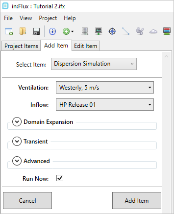
Tutorial 2 - Figure 08 - Setup for the dispersion simulation of HP Release 01 on a Westerly wind
-
Leave the Mesh Expansion and Transient options alone for now. These are discussed in the Advanced Capabilities and Tutorial 8 sections, respectively.
-
Make sure the Run Now checkbox is selected and click the Add Item button.
After clicking the Add Item button the following text will appear in the panel below the Add Item button indicating that the dispersion simulation has been added to the project. It will then be listed in the Dispersion Simulations header in the Project Items tab.
![]()
Tutorial 2 - Figure 09 - Displayed text when dispersion simulation is added to the project.
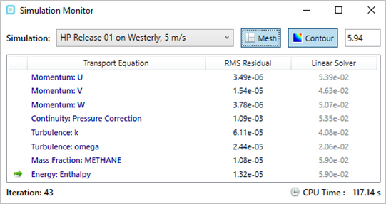
In the same way as the ventilation simulation, after initialization and meshing, a green progress bar will appear next to the item name in the Project Items tab, as in Figure 10. The text of the dispersion simulation will remain gray until the calculation is complete.
Tutorial 2 - Figure 10 - Indication of HP Release 01 on Westerly wind simulation listed in the Project Items Tab with 2% completion
CFD calculations for dispersion generally take longer than the ventilation simulations due to the additional variables being solved, such as the mass fraction of the dispersed gas. During the simulation we will position the 3D window to view the calculation in progress and look at two new variables in the simulation monitor:
-
Right-click in the 3D window and select Top View from the View From option.
-
Press Ctrl+P to change to an orthographic view or choose Orthographic from the Projection option in the same view menu.
-
Double click the dispersion case listed in the Project Items Tab to open the simulation monitor and click the mesh button (
 ), your 3D window should appear as Figure 11 below.
Tutorial 2 - Figure 11 - Top orthographic view of mesh at start of dispersion simulation - 10% completion
-
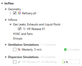
Notice that the simulation monitor now has two additional variables listed in the Transport Equation column: Energy: Enthalpy, and Mass Fraction: METHANE
Tutorial 2 - Figure 12 - Simulation Monitor for HP Release 01 dispersion simulation.
-
You can click on the any equation to preview the currently calculated values. NOTE: these are not the final results. Zoom into the leak location and click the Mass Fraction: METHANE text in the Simulation Monitor. The contour height will be set to "5.94", this value is automatically set from the elevation of the defined leak, but you may enter another height if desired. The contour previewed in the simulation monitor can only be on the XY plane. Below, we can see that the mesh is very refined around the leak source and more coarse further away from it. This keeps the accuracy high and run times low. The mesh and contours will continue to change and adapt as the calculation progresses.

Tutorial 2 - Figure 13 - Screenshot showing a preview of the contour of Mass Fraction of Methane with the initial mesh refinement at 50% completion
-
While the simulation progresses, take some time to have a look at the other transport equations in the Simulation Monitor. Zoom out, while still displaying the mesh and mass fraction contour from the simulation monitor. As the calculation progresses the RMS Residuals will lower and also the mesh downstream will also refine, as shown in Figure 15.
-
The simulation will progress calculating each of the transport equations until completion, which will be around iteration 400. At this point in:Flux will go into a "Finalizing" mode of the calculation as shown in Figure 14 below. During this mode, extra iterations are run to further refine the mass fraction calculation of the dispersion. The green bar will indicate how close to completion the calculation is.
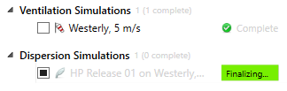
Tutorial 2 - Figure 14 - Project Items panel showing the 'Finalizing' phase of the calculation
-
Let the simulation fully complete, this will be representation by a green checkmark (
 ) next to the dispersion simulation. You have now finished
your first dispersion simulation with in:Flux!
) next to the dispersion simulation. You have now finished
your first dispersion simulation with in:Flux!
Calculation times will vary depending on how many available CPU cores are on your machine. in:Flux is parallel by design and will use all cores available for calculating results. Generally speaking, the more cores you have, the faster the calculation.

Tutorial 2 - Figure 15 - Screenshot of the mesh refinement after the simulation has completed.
Once the simulation is complete, continue to the next section where a new type of post-processing visualization will be added.