‎ Changing Isosurface Parameters

 

For this tutorial we will switch the simulation linked to the already defined isosurfaces. The isosurfaces can be changed to any completed dispersion case, rather than adding separate isosurfaces (one for each dispersion).

 

It is user preference as to how you want to maintain your in:Flux project. Some users may prefer to add a new isosurface for each case they are interested in viewing, while other may have one isosurface used in relation to a single variable and then change the simulation it references.

 

As two isovolumes are already defined and we have the same gas in all three of the leaks, we can move both isosurfaces at the same time to a new leak:

1. From the Project Items tab, right-click the Isosurfaces header text

2. In the menu that appears, choose Set All to Simulation

3. All the completed simulations will appear in the next menu, choose HP Release 03 on North-Easterly 5 m/s as indicated in Figure 31.

 

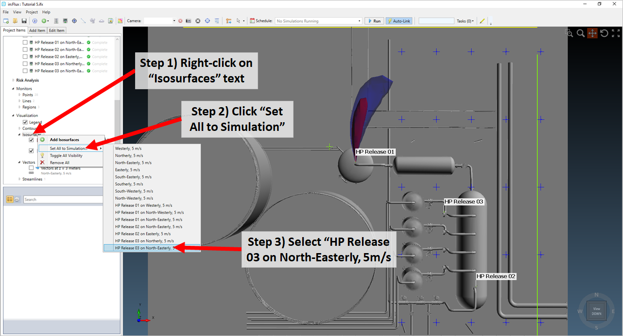
Tutorial 5 - Figure 31 - Indication of how to change the simulation associated with the already defined 100% LFL isosurface

 

in:Flux will then need a moment to extract the simulation data from memory. Once finished your 3D window should appear as Figure 32 and 33 below with the two defined isosurface coming from the HP Release 03 location. Figure 33 shows that the momentum of the release defines most of its shape for the higher 100%LFL concentration but the wind has more effect on the 50%LFL isosurface, this will become more apparent at lower concentrations as the wind will overpower the momentum of the release.

 

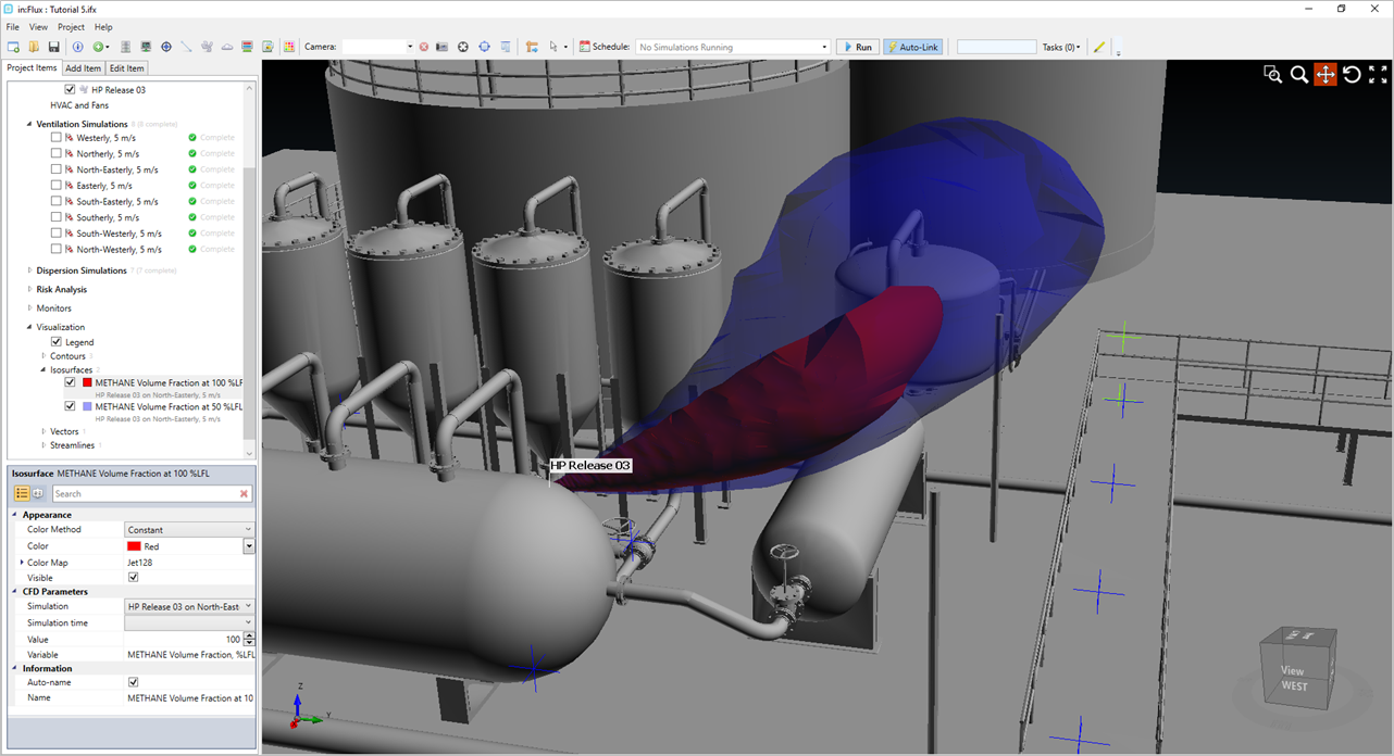
Tutorial 5 - Figure 32 - Showing the 100%LFL (red) and 50%LFL (blue) isosurfaces moved to HP Release 03

 

 

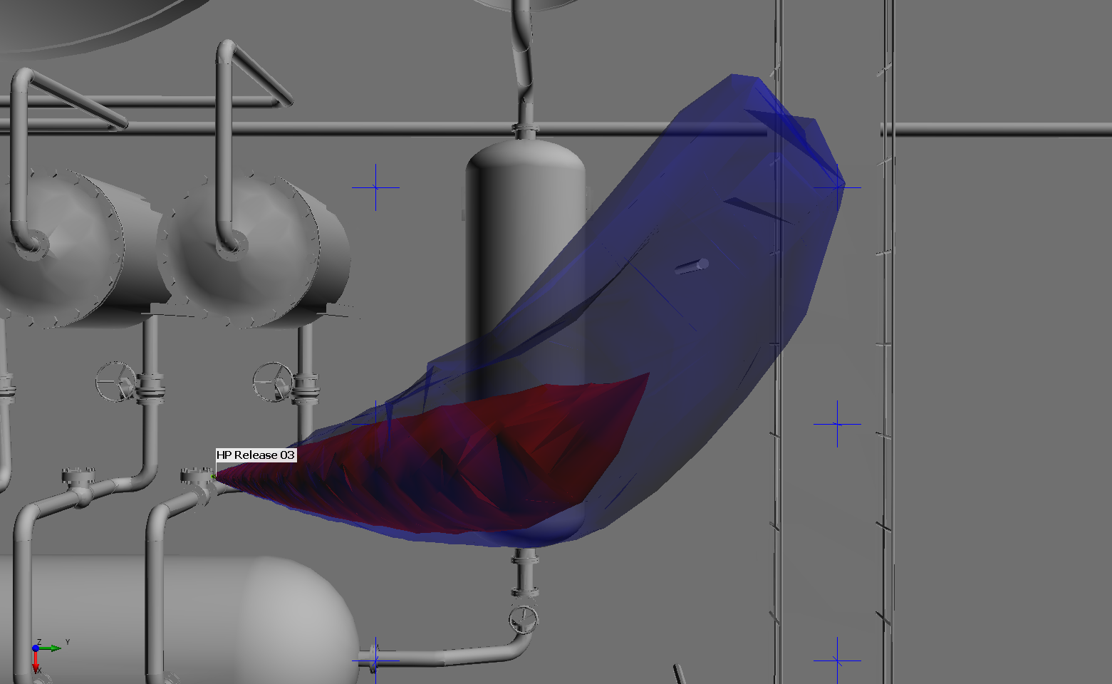
Tutorial 5 - Figure 33 - Isometric view of the 100%LFL and 50%LFL isosurfaces for HP Release 02 with the North-Easterly wind case

 

The value of the isosurface parameter can be changed after it has been defined. For our example, change the transparent blue 50%LFL isosurface to a 25% LFL isosurface using the following steps:

1. Selecting the METHANE Volume Fraction at 50%LFL name from the Project Items tab.

2. Under CFD Parameters, change the Value by highlighting the number 50 and entering a new value of "25" as the %LFL, as indicated in the figure below.

    

   

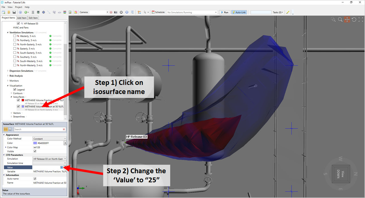
   Tutorial 5 - Figure 34 - Indication of where to change the value associated with an already defined isosurface

    

3. Click in the 3D window to confirm the new value. After a moment of extracting the data from memory, the isosurface will be updated and appear similar to the Figure 35 below. The screenshots were taken by right-clicking in the 3D window and selecting Copy to Clipboard and choosing a white background.

 

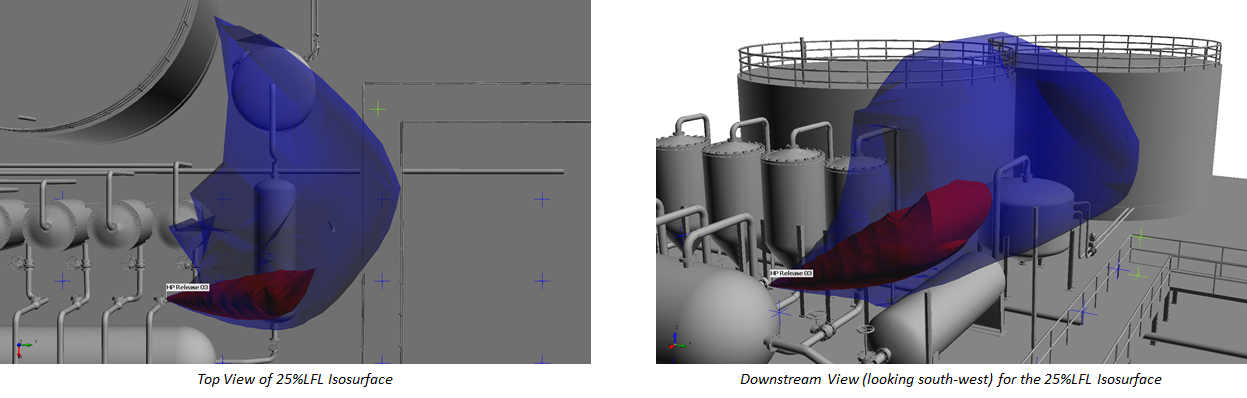
Tutorial 5 - Figure 35 - Updated in:Flux window displaying the 25%LFL isosurface for HP Release 03 on Norther-Easterly, 5m/s wind

 

From Figure 36 we can visually confirm some of the numerical data we received from the gas cloud analysis and monitor points (discussed in the last section). At the lower 25%LFL concentration the north-easterly wind overpowers the momentum of the leak and pushes the cloud back onto itself resulting in a larger accumulated cloud producing the higher gas cloud volumes seen in the Gas Cloud Analysis Window.

 

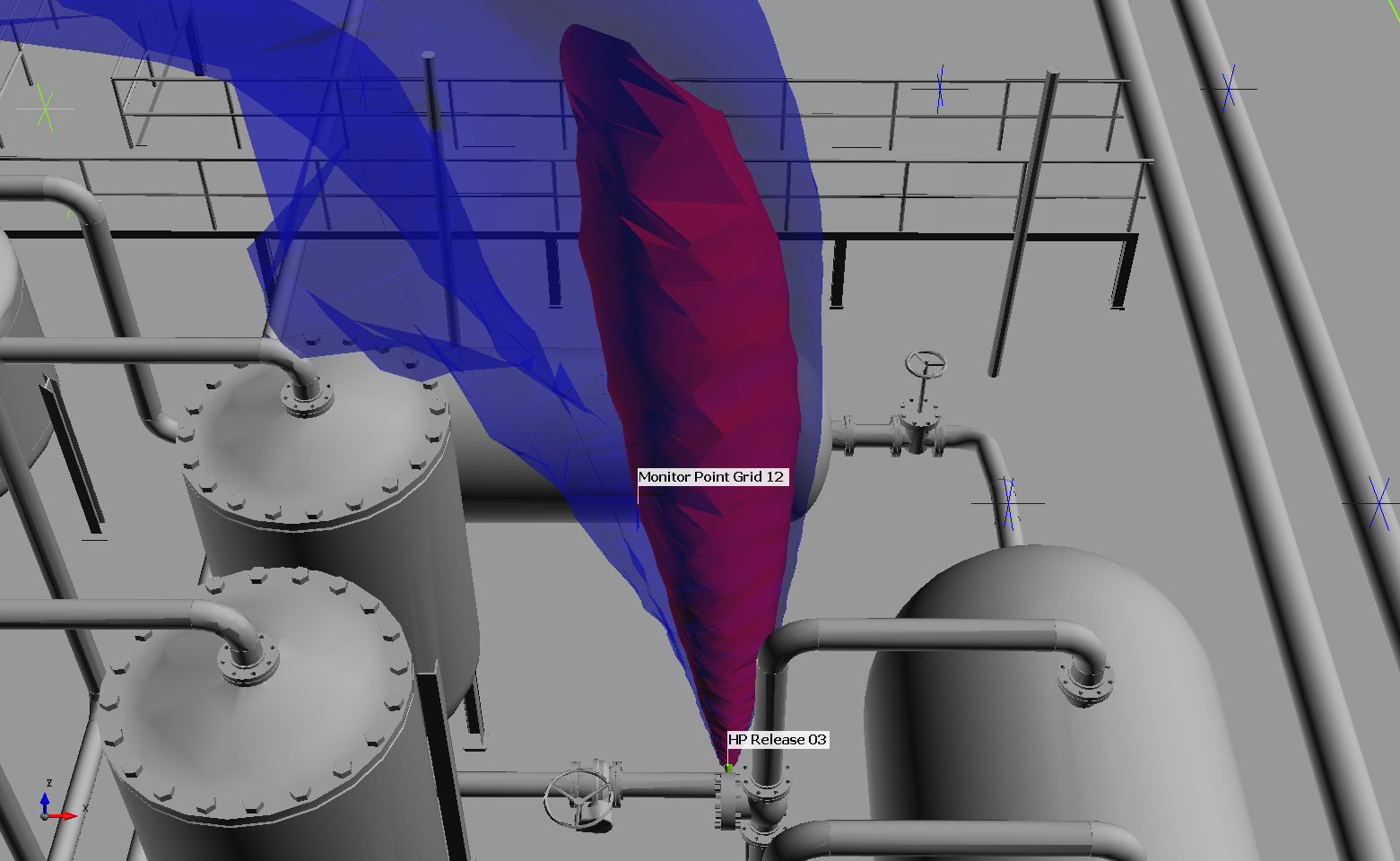
Tutorial 5 - Figure 36 - Showing Monitor Point Grid 12 residing within the 100%LFL isosurface confirming the concentration obtained in the last section

 

Repeat the first Steps 1 - 3 (Figure 31) and move the isosurfaces to HP Release 02 on North-Easterly 5 m/s. The resulting 3D window should be similar to Figure 37 below. Using this capability is useful when looking at the results for several simulations. For projects with several cases, you may opt to use the batch image output to generate an image for each simulated case with the chosen visualization (e.g. %LFL isosurfaces). See Tutorial 6 for more details about the Batch Image Output capability.

 

 

Changing the isosurfaces to the HP Release 02 case shows that the 100%LFL isosurface is not affect much by the wind - the momentum of the leak takes precedence much more so than the case in Figures35 and 36. The 50%LFL isosurface is pushed back on itself because of the wind in the opposing direction. For our purposes, this would result in the cloud traveling above the equipment and flanges of the facility and thus perhaps would not be as much of a worst case scenario as initially anticipated. Feel free to go back and have another look at additional combinations of leaks and ventilations that would result in larger gas clouds.

 

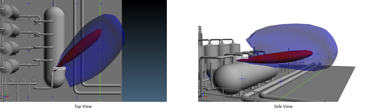
Tutorial 5 - Figure 37 - Resulting image from changing the isosurfaces to link with HP Release 02 on North-Easterly 5 m/s

 

Using the knowledge that you have gained add a third isosurface of 10% concentration and try to recreate Figure 38 below which confirms that lower concentrations of the HP Release 02 on the North-Easterly wind is carried past the flanges and valves of the facility.

 

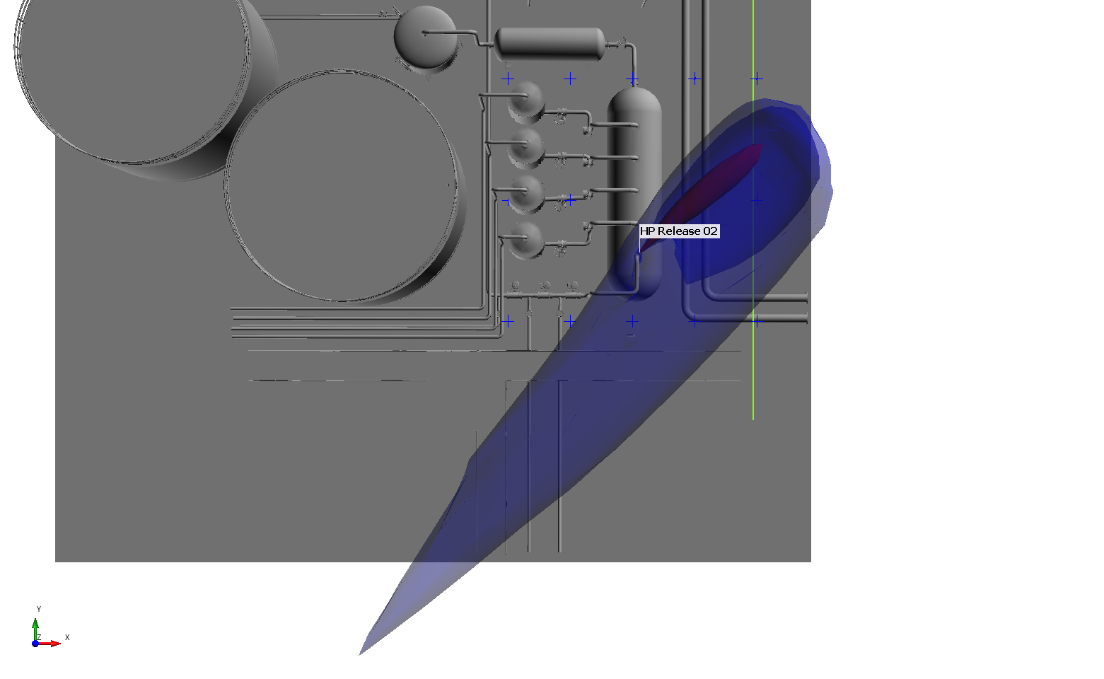
Tutorial 5 - Figure 38 - Screenshot image to recreate for HP Release 02

 

Take some time to change the isosurfaces to the other simulations. Which do you think would be considered a worst case? Is more analysis needed? Generally, when performing CFD analyses, after running a couple of test cases, several more variations on those initial cases are examined.

 

After performing the above, you should have a grasp on changing the simulation associated with an isosurface. The same process can be used to change the simulation for contours, vectors, and streamlines.

 

Congratulations! The simulations you just performed is equivalent to over a week of work using other CFD software.

 

As a reminder, the previous two sections of Tutorial 5 aim to show you that there are various ways to manipulate and display the post-processing visualizations. There is no need to have one isosurface or one contour for each calculated simulation, it becomes a personal preference on how you want to organize and convey the results.

 

When you are done reviewing the results save your Tutorial 5 file.