Adding an Isosurface
An isosurface is a three-dimensional region representing the value of a specific variable in the simulation. For in:Flux this visualization is typically used to indicate regions of specific concentrations of gas shown as percent volume, percent LFL, or percent UFL. However, several other variables can also be shown.
In this tutorial a 100% LFL and a 50% LFL isosurface will be added.
-
Click the Add Item tab and select Isosurface from the dropdown menu.
-
Leave the name to its automatically generated one.
-
Select the HP Release 01 on Westerly, 5 m/s as the Simulation.
-
Set the Variable to be METHANE Volume Fraction, % LFL from the dropdown menu. There are several other variables to choose here, ranging from velocity magnitudes to temperature values. You may also choose the Flammable Gas Volume Fraction, %LFL here for the same result. This variable (described more here) looks at just the flammable components of the gas release, as this dispersion is a pure methane leak the results will be the same.
-
Enter a value of "100" as the %LFL Value.
-
Set the color to be Red by selecting the red swatch (
 ) from the available color palette dropdown menu.
 -
Click the Add Item button to add the 100%LFL isosurface to the project. Your 3D window should show the red isosurface of the plume that is pointing away from the large tanks and towards the walkway, similar to that in Figure 16 below.
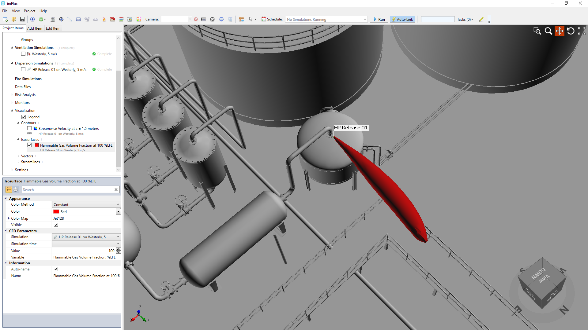
Tutorial 2 - Image 16 - The 100% LEL plume from HP Release 01 dispersion simulation added to the project
-
Repeat steps 1 through 4 above, but this time change the %LFL Value to "50".
-
And set the Color to a transparent blue:
-
Click the Color dropdown menu and select the blue swatch from the available color palette
-
Click the Color dropdown menu again and click the Advanced button at the bottom of the color palette dropdown menu
-
Four horizontal bars will appear, shown in Figure 17, corresponding to the red, green, blue, and alpha values of the chosen color. The alpha value (labeled - A) represents the transparency of the object. Move the scroll bar on the Alpha channel to a value of "100" which will increase the transparency of the isosurface to be added to the project, a value of 255 will results in a sold, fully opaque, color.
-
Click anywhere off of the color palette dropdown menu to confirm the transparent color
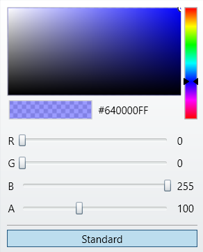
Tutorial 2 - Figure 17 - Advanced color palette menu showing a value of 100 for the Alpha channel, making the color transparent
-
-
Click the Preview checkbox to see the isosurface is now larger and is transparent as in Figure 18 below.
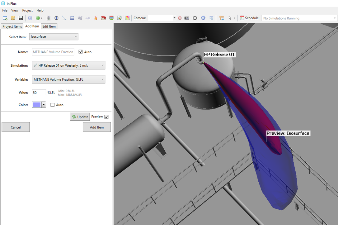
Tutorial 2 - Image 18 - Image of the 50% LFL plume from HP Release 01 dispersion simulation
-
Click the Add Item button.
The plume has a slight bend in the westward direction due to the effect of the westerly wind traveling around the large tank. The momentum of the release has the most effect of the direction of the flow but as the distance away from the leak source increases the flow becomes more affected by the wind.
Updating the Offset Height of an Already Defined Contour
If we look at the streamwise velocity contour defined in Tutorial 1, we can verify that the higher wind velocities occur where the LFL plumes exist. For this example, we will move the streamwise velocity contour from its initially defined height to be at the same height as the release, 5.94 meters, to view the velocities at that height.
To edit the contour height:
-
Select the 'Streamwise Velocity at z = 1.5 meters' text in the Project Items tab.
-
In the properties panel, located at the bottom left of the screen, under the Information section, change the Plane Offset value by highlighting the '1.5' text with your mouse cursor and then entering a value of "5.94" as a replacement, as shown in Figure 19 below. Note - You MUST click off the panel to verify the newly entered number.
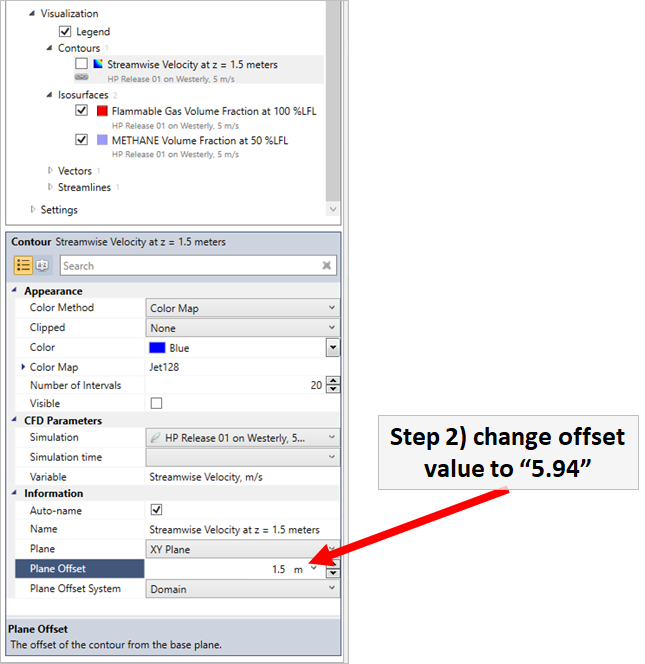
Tutorial 2 - Figure 19 - Indication of where to change the height of the streamwise velocity contour
-
Click anywhere within the 3D window to confirm the new height of the contour. The contour name will change to 'Streamwise Velocity at z = 5.94 meters' and briefly turn gray as in:Flux pulls the data from memory to update the visual.
-
Turn on the visibility of the contour by clicking the checkbox next to the 'Streamwise Velocity at z = 5.94 meters' name in the
-
If the legend doesn't appear, right-click the 'Streamwise Velocity on XY plane at z = 5.94 meters' text in the Project Items tab and select Link to Legend, as shown in Figure 20. This will change the displayed legend to reference the ranges of the contour.
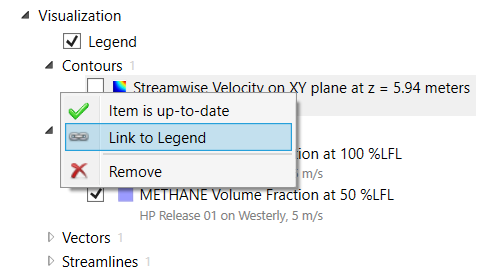
Tutorial 2 - Figure 20 - Context menu for selecting Link to Legend after user right-clicks on the contour.
Your in:Flux window should appear similar to Figure 21, verifying that higher wind velocities exist in the flow where the isosurfaces start bending. More information on what capabilities are available for contours is discussed in Tutorial 6.
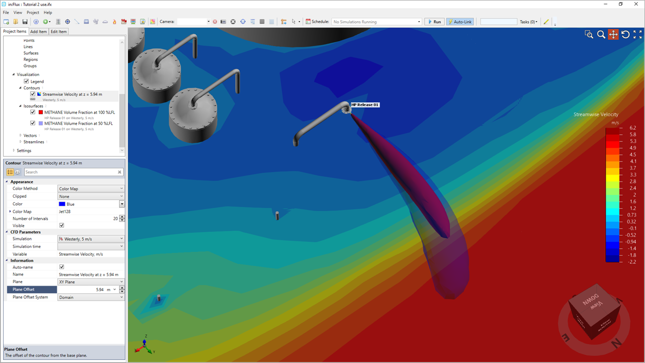
Tutorial 2 - Figure 21 - Streamwise velocity contour showing negative flow (shown by dark blue regions) and faster flow (shown by orange and red regions)
Multiple contours can be added to each project and show data from dispersion or fire cases as well as ventilation ones. Continue to the next section to add a second contour to the project.