‎ Editing Post-Processing Visuals

 

Once a simulation has completed, all of its associated data is stored in the memory of your computer. This allows for you to add post-processing visualizations after the calculation has finished.

 

Tutorial 4 added several ventilations to the project, we will examine these simulations by looking at a contour of the streamwise velocity for a selection of cases to assess where re-circulation and stagnant flow exists in our example. Doing this is helpful in determining which combination of leak locations and wind directions are relevant for a particular application. Otherwise every combination of wind direction with all leak locations would need to be simulated, which is a tedious process but not impossible.

 

A new visualization does not have to be added for each dispersion case, instead we can change the data that is linked to the already defined contour:

1. Change to a Top View in the 3D window by selecting it in the view cube or by the View From option when you right-click in the 3D window, press Ctrl+P to change to an orthographic view.

2. In the Project Items tab select the 'Streamwise Velocity on XY plane at z=5.94 meters'

3. In the Properties Panel change the Plane Offset to "5.5" meters and click anywhere in the 3D window to confirm the change. This moves the contour to the height of the HP Release 02 location.

    

   

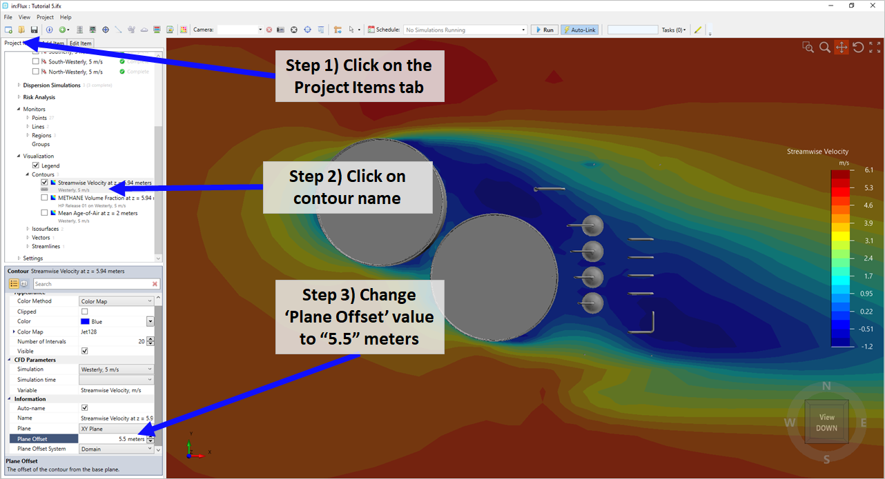
   Tutorial 5 - Figure 14 - Steps for changing the Westerly wind contour height

    

4. In the same properties panel of the same contour, change the Simulation to Northerly, 5m/s under the CFD Parameters header, as shown in Figure 15 below. Click within the 3D window to verify the selection. A window may appear for a few seconds to notify you that in:Flux is retrieving the simulation data from memory.

    

   

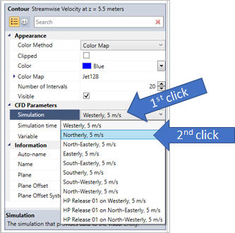
   Tutorial 5 - Figure 15 - Changing the simulation linked to the already defined contour

    

   The resulting Figure 16 shows that the northerly wind has faster speeds along the eastern and western edges of the facility. As a reminder, to replicate Figure 16, you will need to right-click on the 'Streamwise Velocity on XY plan at z = 5.5 meters' and choose Link to Legend. It is known that the higher wind speeds will disperse the gas away from the equipment and thus may not be considered as much of a worst-case scenario for HP Release 02. However, for HP Release 03 we can see that the higher speeds are nearby to where the gas plume may exist and develop. This is because the release location is at a 3 meters height but is angled 15 degrees upward so there is high likelihood of the plume existing in this region with the higher wind speeds.

    

   

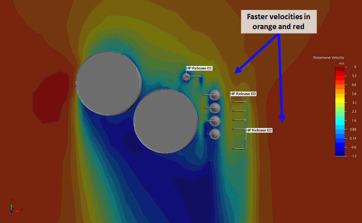
   Tutorial 5 - Figure 16 - View of the Northerly wind contour at a 5.5 meter height. Legend has been 'linked' to the contour

    

5. Repeat Step 4 and switch through the other ventilations in the Simulation dropdown menu. Which wind direction would result in a worst-case scenario where the gas from HP Release 02 would accumulate the most? A selection of different ventilations is shown below.

    

   

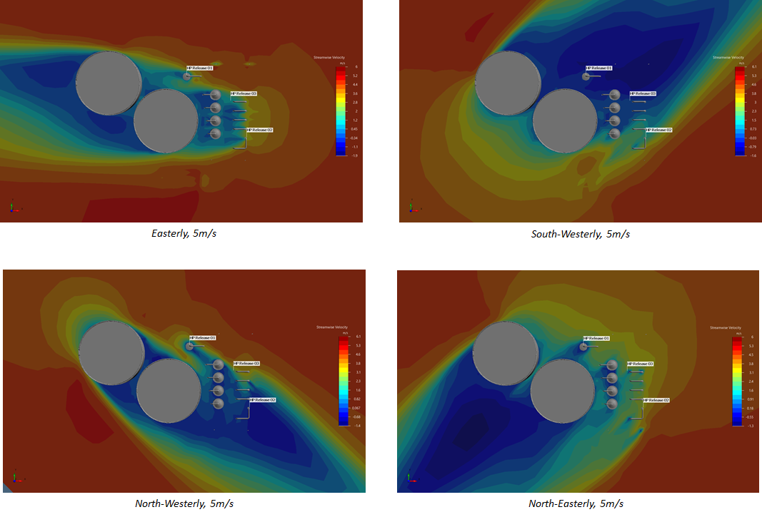
   Tutorial 5 - Figure 17 - Four views showing contours placed at 5.5 meters height for varying wind directions

    

6. In the same way, we can change the simulation the vectors are showing from the properties panel. Vectors give more indication to the actual direction of the flow rather than just a color representing wind speed. Turn off the visibility of the contour and turn on the visibility of the vector field in the Properties Panel. Change the Simulation referenced by the vectors in the properties panel as shown in Figure 18. Choose the North-Easterly, 5 m/s simulation to view first.

    

   

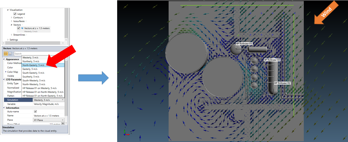
   Tutorial 5 - Figure 18 - Changing the simulation shown by the vectors defined in Tutorial 1

    

7. The offset of the plane is still set as 1.5 meters from the ground, as was defined in Tutorial 1. Take some time and look at different elevations (changing them as in Step 3 and Figure 14 above for the contours via the Plane Offset) with various wind simulations (changing them as in Step 4 and Step 6). Which of these confirm or deny your thoughts from the contours of Step 5? A selection of screenshot of vectors is shown below.

    

   

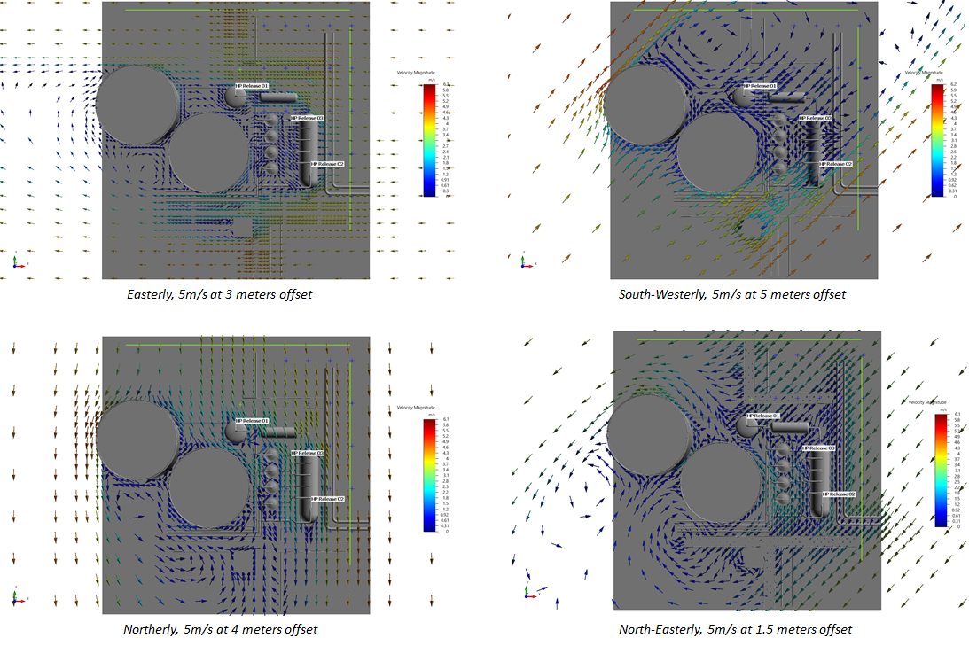
   Tutorial 5 - Figure 19 - Views of vector fields at different heights for a range of ventilation cases

    

8. Reviewing the figures in this section:

   1. For both HP Release 02 and HP Release 03, the north-westerly and south-westerly wind direction has lower wind speeds near the releases.

   2. However, for HP Release 02, both the easterly and north-easterly winds blow in a direction that would carry the gas toward process equipment and other vessels. It can also be argued that the south-easterly direction may also be a valid case. For simplicity, only the easterly and north-easterly cases will be examined for the HP Release 02.

   3. With the same argument as in part b) above, for HP Release 03, it can be said that the northerly, north-easterly and north-westerly winds flow against the leak direction and back towards all the flanges and valves of the facility. For this tutorial we will look at the northerly and north-easterly wind directions for HP Release 03, but you may simulate more cases if you choose to.

   4. In summary, 4 dispersion simulation cases will be set-up in the next section based on the above information:

      1. HP Release 02 on Easterly, 5 m/s

      2. HP Release 02 on North-Easterly, 5 m/s

      3. HP Release 03 on Northerly, 5 m/s

      4. HP Release 03 on North-Easterly, 5 m/s

 

You may choose to simulate more cases than this on your own, but for the purposes of this tutorial only the four simulations mentioned above will be examined.

 

The problem in Tutorial 5 may also be approached by using Risk Data. The Risk Based Simulations Tutorial provides instructions for how to setup 100s to 1000s of cases to generate a consequence map of where the highest risk of combustible gas is present considering all the dispersion and ventilation cases simulated. 

 

Continue on to the next section to set up and run the four dispersion simulations.