Risk-Based Gas Mapping Workflow
The below is a short summary of the suggested workflow for performing risk-based gas mapping (RBGM) analysis using in:Flux CFD software. This approach conceptually has existed for several years but has only recently been made available to consultants and engineering firms without the use of super computers or clusters as using in:Flux and the ifx:Solve software enables 1,000s of CFD cases to be solved in just a couple of days.
A PDF version may be downloaded here.
Planning and Preparation
Input Data Checklist
Much of the time spent in the initial phase of a RBGM project is locating, and generating, the input data. Below is a list of items to gather prior to starting the project:
-
3D CAD Model (DGN or Navisworks files preferred)
-
QRA or FERA document, if available, or other data categorizing the hazards associated with the modules/regions for analysis
-
Parts List with inventory and leak frequencies
-
Wind Rose and Environmental Conditions
-
Location, size and flow rate of forced ventilation/fans (if any)
-
Coverage or risk-reduction target, typically from end user
-
Existing Detector layout (if any)
Geometry Setup and Simplification
A typical RBGM project includes thousands of CFD simulations, so it is well-worth taking time to simplify the geometry as this can significantly reduce computation time of the entire project.
For very large geometries, consider dividing the project by module. Use the Crop Tool so that the detailed geometry is included around the module, but far-field items are represented
more coarsely, either using porous regions or creating simple 3D CAD. Occasionally,
far-field geometry can be ignored. Sensitivity studies can be performed on the geometry simplification to check that there are no significant differences between using the full model and the simplified model.
Verify if your site has grated decks or plated decks and check these against your CAD model and, if necessary, add porous regions to replace plated decks.
It is often useful to run a few sample ventilation and dispersion cases to check that the gas clouds form as expected and test performance. Ideally, the run-time for ventilation simulations should be less than 10 minutes, and for dispersion simulations,
less than 30 minutes. The maximum run-time for a single dispersion simulation should be roughly 60 minutes.
Scenario Selection
It is impractical to run every combination of leak location, direction, hole size and wind condition. An important part of the project is narrowing down the number of cases to reduce the total computation time of the project.
Leak Locations and Frequency Data
Guidance for leak locations and wind data should come from the QRA, if available. The QRA should indicate equipment of medium and high risk as well as the frequency of gas leak for various hole sizes. If this information is not available, the OGP Directory for Process Release Frequencies can be used.
Equipment Grouping
It is often useful to group equipment that are close together. The modeled leaks are then representative of all leaks from the equipment in the group. The total leak frequency from the group can be summed from the individual components.
Note that the release frequency can vary by two or three orders of magnitude depending on type of equipment. Modeling leaks from equipment with very low leak frequency will make little difference to the results of a risk-based analysis and can
be ignored in certain circumstances.
Determining the Hole Size
From each equipment item (or group), the modeled hole size should be determined. It is often only necessary to simulate one hole size - the smallest hole size that presents a significant consequence. Leaks smaller than this size, while being more frequent, do not generate gas clouds large enough to present a significant explosion risk. By contrast, leaks larger than this size are less frequent, and can be assumed to be detected as the resulting gas cloud is larger than the one used in the study.
The critical gas cloud size to evaluate can be determined by the consequence modeling performed in the QRA. If this information is not available, it is recommended to use a cloud volume equivalent to that of a 6-meter diameter sphere. This volume
is the one determined by the OTO 93-002 report as being the smallest to generate overpressures greater than 150 mbar in congested (typically offshore)
environments. Using this cloud volume for onshore project, where the congestion is lower and thus the expected overpressure is reduced, is a conservative assumption.
The hole size necessary to generate a 6m diameter gas cloud depends on the process conditions and gas composition. It is typical for the flow rate to be in the region of 3-5 kg/s for hydrocarbon leaks, which is roughly 20-50 mm for many process
conditions. It is highly recommended to perform several dispersion simulations to confirm that the chosen hole size is appropriate to generate the critical gas cloud size. The target flammable gas volume is around 113 m3.
The gas cloud volume will vary greatly depending on leak location and wind conditions, but the goal is for the average flammable gas cloud volume to be in the range 50-100 m3, this
can be checked using Monitor Regions.
It is normal to simulate one hole size for each equipment item, but to vary the hole size depending on process conditions – high upstream pressures will require smaller hole sizes to generate significant flammable gas clouds than low upstream
pressures. Indeed, it may be the case that the pressure and composition may be such that it is impossible to generate large flammable clouds from certain equipment items. If this is the case then it can be argued that these items do not present a
significant explosion risk, and thus do not need to be modeled in the analysis.
Note that many problems with RBGM projects arise from modeling too small a hole size, from the mistaken belief that only frequency matters, and therefore the hole should be as small as possible. It is important to remember that risk is a combination
of both frequency and consequence, and, when performing RBGM, the risk of interest is explosion risk. Very small leaks that generate small gas clouds often present little or no explosion risk.
Leak Directions
Once the leak locations and hole sizes have been determined, the leaks should be added to the project. This involves adding specific leak sources to each equipment item.
It is very important that the sum of all the individual leak frequencies should equal the total leak frequency of the equipment item. For example, if the leak frequency of a flange is 1 x 10⁻³ and four directions are modeled, then the individual leak frequency is 2.5 x 10⁻⁴.
Note that leak frequencies can be modified after the project is completed without needing to rerun the CFD simulations. Errors in defining the leak frequency can be corrected easily.
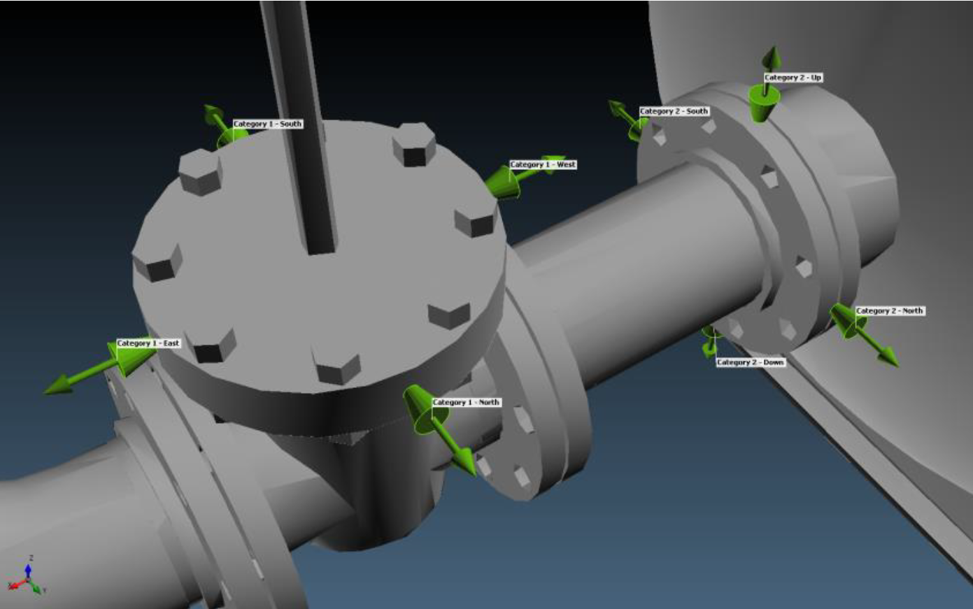
It is standard to consider four leak directions for each location, but more can be added as necessary.
Environmental Data / Wind Rose
Environmental data should be available from the QRA or other data source. It is common to group the data into 8 or 12 wind directions, and 2 or 3 wind speeds.
Total Simulation Count
Throughout the setup process, keep in mind that additional leak locations hole sizes, wind speeds or wind direction can significantly increase the number of cases to be run. The total simulation count will vary on a project basis, but typically the number of modeled scenarios should be in the range of 1,000 to 3,000 per module.
Note that it may not be necessary to model all the scenarios that have been defined in the project. A leak that has a low frequency, combined with a low-probability wind condition, may be 2 or 3 orders of magnitude lower frequency than
other scenarios. Modeling these low-frequency scenarios may not be necessary, as even if the gas is assumed to be undetected, it would not significantly reduce the coverage of the layout.
The Gas Detector Optimization capabilities of in:Flux always calculate coverage based on all of the scenarios defined, regardless of whether they are
modeled or not. Any scenario that is not modeled is assumed to be undetected.
Project Setup
Gas Composition Definition
Single and multi-component gas compositions should be defined for each inventory first, so that they can be used when defining leaks.
Leak Definition
The Risk Manager's leak frequencies tab can be used to define leaks individually or groups at a time. Properties of the leak (e.g. location, direction, hole size, composition, frequency, etc) are displayed in tabulated form for ease of editing.
Leaks commonly occur on valves or flanges. It is typical to define a set of four leaks around these objects as shown below, although more leaks can be defined.
The Properties editor at the bottom of the Risk Manager window can be used to edit the properties of leaks in bulk or make copies of sets of leaks. The Copy feature is a very powerful function as all the leaks in the project can be selected and then duplicated with different properties. Alternatively, the copy function may be used with the position option in the properties editor to duplicate sets of leaks to nearby or similar flanges or equipment pieces.
Frequency values can be entered in the Risk Manager for each leak individually or divided across a set of leaks using the Cumulative Frequency option. Time should be taken here to accurately define each leak location and direction.
Wind Rose Definition
Wind direction and speed probability values can be entered for up to 12 wind directions. However, each wind direction and wind speed defined will significantly increase the number of simulations run, as described previously. It can be beneficial to perform some initial dispersion cases to determine sizes of gas clouds produced for various wind conditions. This information can then be used to justify a smaller set of wind directions and speeds for the project.
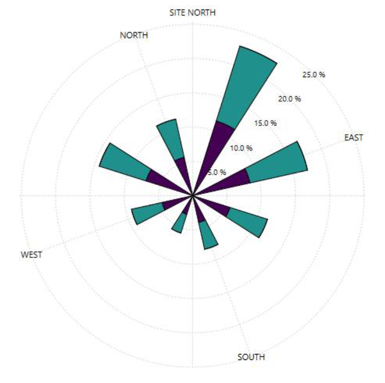
Take care to ensure that the proper offset is set that defines the difference between the Site North and True North. The 3D CAD files are almost always oriented to Site North, while the environmental data is almost always orientated to True North.
It is much easier to manage the project using the Site North orientation, so the wind rose should be rotated, as in the example below.
Simulation Summary Review
Once leaks and wind cases are defined they combine to make the dispersion cases of the project and are listed in the simulation summary. Exporting this table to Excel is recommended so that all of the information entered can be double checked before starting the calculations.
In the simulation summary table, each column can be sorted so you may determine that only cases above a certain frequency should be simulated (this is only possible if frequency information is entered for each defined leak). Use Ctrl and/or Shift
keys with the mouse to highlight a sub-set of cases to be added to the project or click the All checkbox to include the entire set. It is suggested to have the Run Now checkbox unselected so that risk data sets and monitor regions can be
defined before calculation starts.
Risk Data Set and Monitor Region Definition
Risk Data Sets are used to combine all the simulated cases for one variable, for RBGM this would be the Flammable Gas Volume Fraction, %LFL. The gas detector optimization will only be performed on the information generated within this region. Post-Processing items such as risk contours will also be limited to the bounds of the Risk Data Set. Having large or multiple risk data sets in the file will significantly increase the file size of the ifx project (>10GB). It is recommended to only have one or two risk data sets per file and for it to be close fit around the module or region of the assessment. When risk data sets are defined users are prompted if a monitor region should be made with the same dimensions, click Yes as the monitor region generates the consequence value used later.
It is important to perform this step before calculations start as if they are defined after simulations are complete it will take several hours to extract the needed information.
Project Calculation
Create Distributed Solver Files and run with ifx:Solve
Rather than have all simulations calculated on one machine, solver files and the ifx:Solve software can be used to distribute the computation of the project to other machines to be run in parallel. This greatly reduces computation time as the computational effort may be distributed over a network of physical or virtual analysis machines. Determine the available computation power you have before deciding on the number of solver files to create.
It is useful to run one dispersion simulation to monitor the resources it requires for a specific machine. Depending on the project and machine, the solve time may be CPU-limited or memory-limited. Based on this first simulation, it should be
clear how many solver files can be run on each machine.
Both in:Flux and ifx:Solve are built in the .Net Framework and will utilizes all cores of the machine for most tasks. However, Windows will manage how much of the processing power is used so it will vary for each machine based on what is going
on “under the hood”. As the license key for ifx:Solve is an unlimited seat type (different from the main in:Flux software license) it allows for an unlimited number of instances to be open and running at the same time.
Updating the main in:Flux project
Upon completion, the solver files (.ifxs) will typically be in the range of 500MB to 20GB each depending on your project. Move them back to the directory which they were created overwriting the original files. Return to the main in:Flux project and choose the Update All option for the data files. This will update all the solver files to reference the completed data. Save the project when this has completed.
Post-Processing
Apply Consequence Values
With the solver files updated, gas cloud volumes for each case will have been calculated. For RBGM, values from the monitor region are used. Check the Gas Cloud Analysis window to ensure the data is present before opening the Consequence Weighting Window. Here you can choose the consequence method deemed most appropriate for your project.
Risk Contour Definition
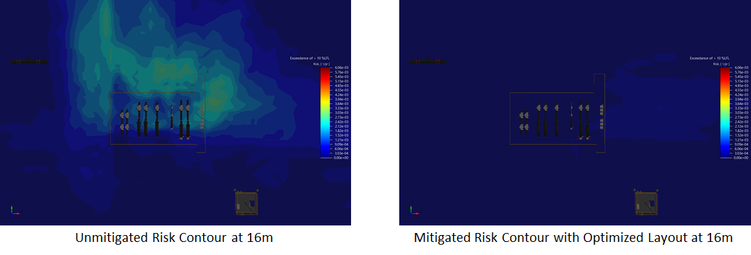
Risk Contours show exceedance values of the variable chosen when defining the risk data set. These risk contours can show results based on three methods: scenario, frequency or risk. For RBGM the third option should be used, as this utilizes the consequence values assigned earlier.
As a point of reference, the unmitigated risk contour of the region prior to performing the optimization can be generated, an example is shown below. Once defined many of these properties, such as the height can be changed so that you can review
the unmitigated risk at different elevations within the Risk Data Set.

After the optimization is performed a new Risk Data Set can be created with all the detected scenarios removed so that a comparison can be made showing mitigated risk vs unmitigated risk. An example image is provided at the end of this document.
Gas Detector Optimization
Plausible Gas Detector Location Definition
Although in:Flux can generate a mathematically optimal detector layout, described later, it is best for users to provide inputs of plausible detector locations. Users will have knowledge of locations for devices based on existing layouts, structural members, wiring racks and other engineering judgement. The more information shared with in:Flux via plausible gas detector locations, the better the optimization will be as a whole.
Monitor Points act as point gas detectors, Monitor Lines act as open path gas
detectors and they can be combined in sets called Monitor Groups. These Monitor Groups can be selected or removed in the optimization controller, which can be useful for comparisons
of existing layouts to the optimal ones.
Perform Gas Detector Optimization
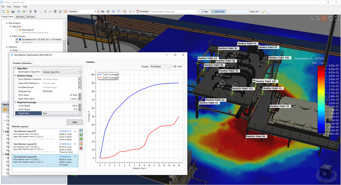
With dispersion cases calculated, consequence values assigned, and detector locations defined, the optimization may now be run. Optimal detector layouts are quick to calculate so you can easily compare different targets, alarm levels or voting strategies. A window showing the optimization controller and the various inputs is below.
Three options are available to select as the Optimization Algorithm for in:Flux and are described here:
-
Greedy Algorithm – this algorithm looks for a defined monitor which will be most effective at reducing the risk. It then adds that monitor to the layout and removes the cases which were detected before continuing and looking for the next monitor which will have the next most effective reduction in risk. The process is continued until the coverage target is met or it cannot improve the layout any further.
-
Optimal Layout – this algorithm provides the mathematically optimal location for point detectors; this does not consider if that location is sensible for installation or not.
-
None – Evaluate Layout – this option only provides the resulting coverage for the layout chosen via the monitor dropdown options at the defined alarm levels. in:Flux will provide the risk reduction (if Risk is set as the Target Basis) for the layout. This is different than optimizing as all of the monitors chosen will be used in the layout rather than in:Flux only selecting the minimal number needed for the coverage targets.
Improve Optimization Results
It may be useful to have a look at the Optimal Layout option as a “first pass” to get an understanding of how many devices may be needed for a module and where plausible gas detector locations may need to be considered. Additionally, once a layout has been generated by the optimization algorithm, a new risk data set can be made and risk contour viewed for the new risk data set which will indicate regions with undetected gas. New monitors can then be placed in these regions and the process repeated several times over eventually converging on an optimal layout.
Export Final Results
Once an optimal layout is chosen, information pertaining to that layout may be exported. A popular option is the Detector Matrix, which produces an excel file showing which scenarios were detected by which detectors in the layout. The rows will be populated with all the scenarios calculated in the project and the columns will related to the detectors in the optimized layout.
The coordinates of the optimized layout can be exported to excel, and the layout may be exported to a Detect3D (.d3d) file.
A powerful image to convey upon completion of the analysis is a risk contour comparing the “before and after” or unmitigated vs mitigated risk of the site with the optimal detector layout, an example image is shown below.